Find 3db Bandwidth Continuous Transfer Function Value Matlab

Introduction to Transfer Functions in Matlab

A transfer function is represented by 'H(s)'. H(s) is a complex function and 's' is a complex variable. It is obtained by taking the Laplace transform of impulse response h(t). transfer function and impulse response are only used in LTI systems. LTI system means Linear and Time invariant system, according to the linear property as the input is zero then output also becomes zero. Therefore if we do not consider initial conditions are zero then linear property will fail and if the property fails then the system will become non-linear. Because of non-linearity system will become Non-LTI system. And for non-LTI system we cannot define transfer function, therefore, it is mandatory to assume initial conditions are zero.

Definition of Transfer Functions in Matlab

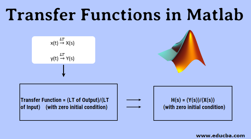
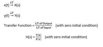
The transfer function of the LTI system is the ratio of the Laplace transform of output to the Laplace transform of input of the system by assuming all the initial conditions are zero.

In the above system, the input is x (t) and the output is y(t). After taking Laplace Transform of the whole system, x(t) becomes X(s), y(t) becomes Y(s) .we consider all the initial conditions are zero because

Methods of Transfer Functions in Matlab

There are three methods to obtain the Transfer function in Matlab:

By Using Equation
By Using Coefficients
By Using Pole Zero gain

Let us consider one example

1. By Using Equation

First, we need to declare 's' is a transfer function then type the whole equation in the command window or Matlab editor. In this 's' is the transfer function variable.

Command: "tf"

Syntax : transfer function variable name = tf('transfer function variable name');

Example: s=tf('s');

Matlab program

2. By Using Coefficients

In this method numerator and denominator, coefficients are used followed by 'tf' command.

In the above example

The numerator has only one value which is "10s", so the coefficient is 10.

And in the denominator there are three terms ", so coefficients are 1, 10 and 25.

Command: "tf"

Syntax: transfer function variable name = tf([numerator coefficients ] ,[denominator coefficients])

Example: h= tf([10 0],[1 10 25];

3. By Using Pole Zero gain

In this method, we use the command "zpk", here z stands for zeros,p stands for poles and k stands for gain.

In above example :

Zeros:

N =0

10 * s =0

(s-0)=0

Here gain is 10 and

s=0

therefore zero present at origin

D= 0

S² + 10s + 25 = 0

S + 5s +5s + 25 = 0

S (s+5) + 5 (s+5) = 0

(s+5)(s+5) = 0

S = -5, -5

Therefore two poles are present at -5.

command: zpk

syntax: zpk([zeros],[poles],gain)

example :zpk([0],[-5 -5],10)

Examples & Syntax of Transfer Functions in Matlab

Below are the various examples of transfer function with their syntax:

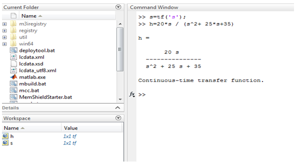
Example #1

The above example illustrated in screen 1 .in this transfer function represented by using equation as well as 'tf' command is used. Values of h and s are stored in the workspace.

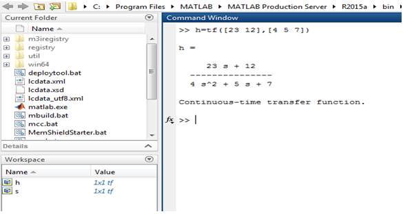
Example #2

In this example, the coefficient method is used. Therefore first we need to find out numerator and denominator separately. Here numerator is 23s + 12 and the coefficient of the numerator is 23 and 12. The denominator is and coefficients of the denominator are 4, 5 and 7

The below image shows the Matlab program for the above example.

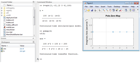
Example #3

In this example input is values of pole, zero, and gain, zpk command is used to find out the transfer function.

Zero's = 1,-2

Pole's = 2,3,4

Gain = 100

It shows output

Advantages

Below are some of the advantages explained.

It is a mathematical model that gives Gain of LTI system. mathematical modeling and mathematical equations are useful to understand the performance, characteristics, and stability of the system
Complex integral equations and differential equation converted into the simple algebraic equations (polynomial equations)
The transfer function is dependent on the System and independent on Input.
If the transfer function of the system is known then the output can be easily calculated.
It gives information about poles and zeros, which can be calculated.

Conclusion

In this article, we have studied various methods to represent transfer function in Matlab which are using the equation, using coefficients, and using pole-zero gain information. In Transfer Function representation we can also plot poles, zero plots by using 'pzmap' command.

This representation can be obtained in both the ways from equations to pole-zero plot and from pole-zero plot to the equation. Transfer function mostly used in control systems and signals and systems.

Duryea Camuctued96